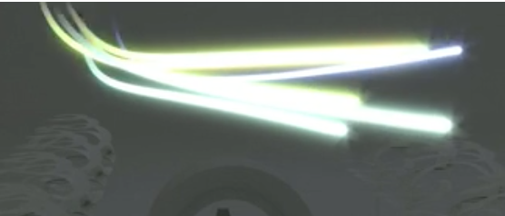
 Path Animation using an animated material on frozen particles. From the last semesters Blender intro week day2 video that’s the technique you can see in the image on the right.
You can download a zip file with a low res version of the video footage here. (58MB)
Go through the file as follows:
Index:
1. Particles
2. Motion Tracking
3. Masking the buildings
4. Masking the trees
5. Animated Particle Materials in Cycles
6. Putting the streets onto the topography
1. Particles (following a path)
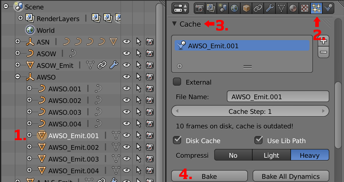
 Go to Frame 500 and play the movie (Alt+A). What you see is two emitters following a path and emitting a particle in every frame. Well, actually there are mostly 4 emitters, each of them emitting its particle at a slightly different offset, but that’s just the hackish workaround to make the particles almost look like a line. If you would like to render this animation you would need to bake the remaining particles first. The zip file you downloaded contains only the baked physics cache for the two paths you see at frame 500. The particles of the remaining particles need to be baked. The cache is located in the folder “blendcache_zurich_view_traffic_web”. To proceed select EACH (not all at once) object containing “Emit” in its name and bake the physics cache as follows:
 Based on your computer’s capabilities this will take maybe half an hour. If you don’t bake the physics you will not find much difference in the rendering process; the particles are simulated on the fly while an animation is rendered out. Nevertheless you need to render the WHOLE animation. If you are rendering only a portion of it you will encounter problems. At least to my experience with Blender <=2.67 many particles behave very strangely and unexpected if you don’t bake them. While the outcome might be considered as a stunning visualization too (look at this video!) you completely loose control over your visualization in some situations. Therefore, bake and be happy.
2. Motion Tracking
Next thing to look at is motion tracking. We use it to link the camera rotation of real and virtual cameras. Furthermore, this is the layout in which you create masks that are composited on top the path animation rendering. The compositing part will follow below.
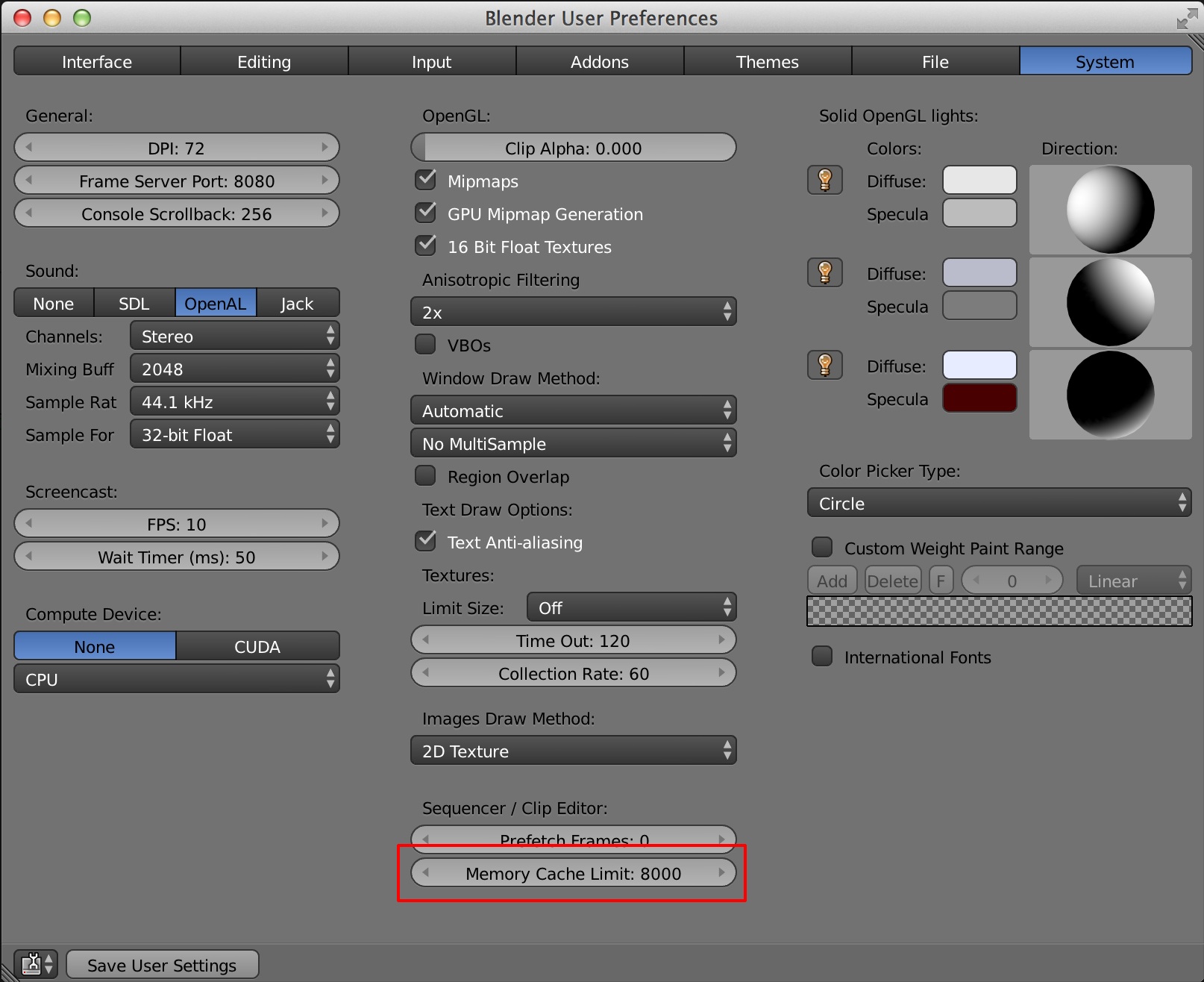
First: make sure you allow Blender to use as much RAM as possible. By default the sequencer, the part of Blender that processes video, is allowed to use 1024MB of your RAM. If you are working on 5 seconds of video this might be enough. Nevertheless, since our video is longer and you probably have more RAM anyway, put this setting to around 5000MB or more, depending on your hardware. Go to File -> User Prefences -> System and adjust the value as shown in the picture below.
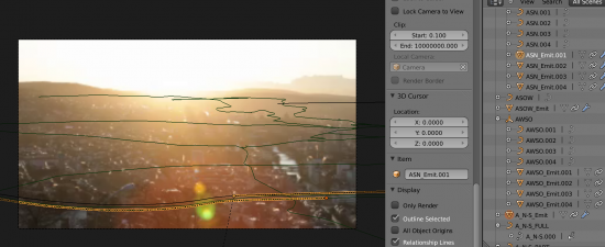
 From the Layout drop down panel (red arrow) choose “Motion Tracking”. Please refer to the Motion Tracking tutorial on our server for the details about setting tracker points. As you can see from this example, even for a camera pan you need many, many tracking points. What you will get out of this is a Blender Camera Object that is rotating with the same speed as your real camera. Remember, the video footage you can download from this website is scaled down to a lower resolution. Don’t try to track any points in this video, since there are not enough pixels.
![]()
Notice the Masks (2) that have been drawn for this movie. We use those masks to cut out the front most buildings and use them to cover our rendered geometry (the animated paths). The masks are drawn as a vector shape and then hooked to a tracker point.
3. Masking the buildings
Now look at the Compositing Layout to see how the masks are being used:
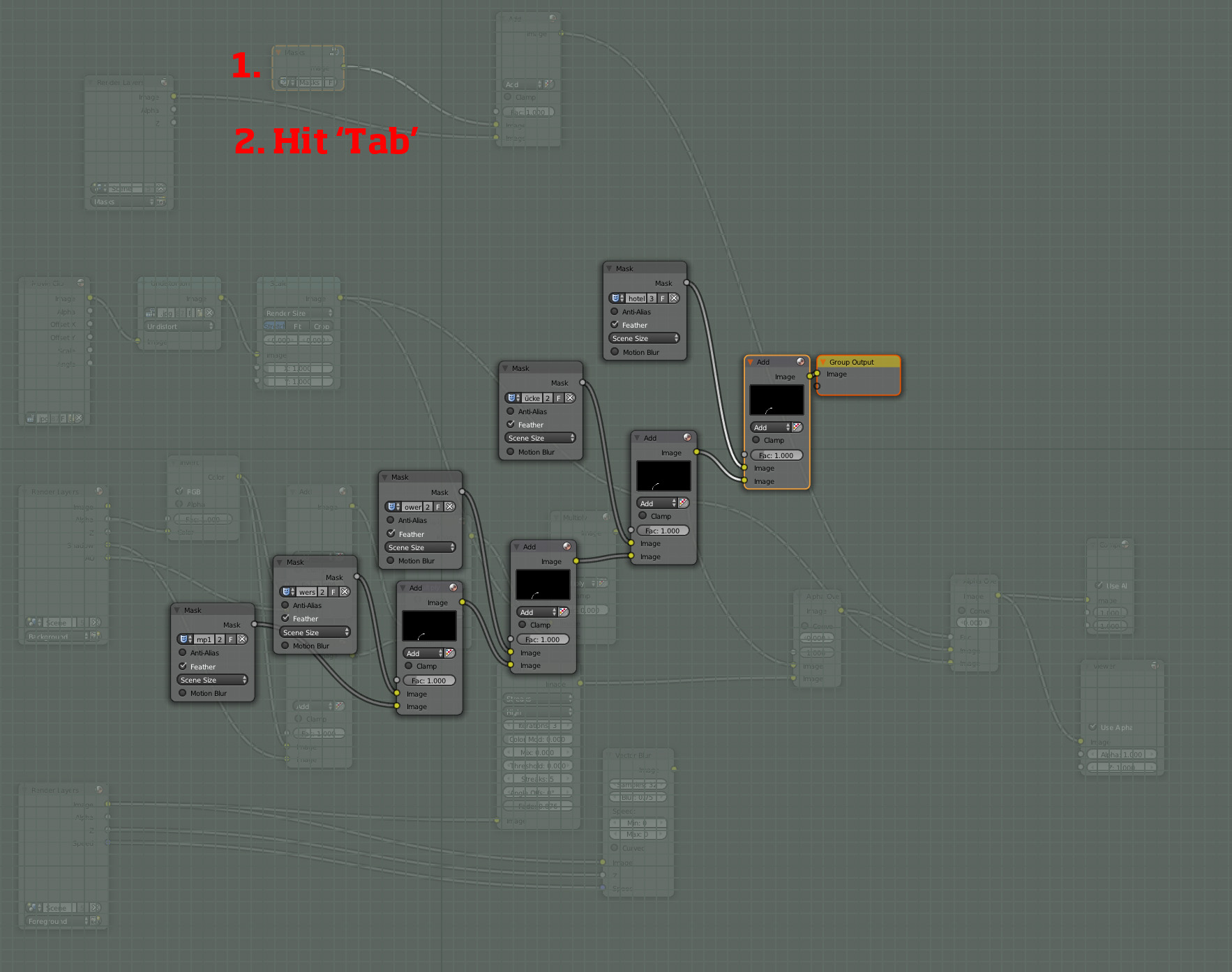 Select the node called “masks” and hit “Tab” on your keyboard. The mask node is a group of nodes. With “Tab” you can “open” the group and see what’s inside. What you will discover in this group is all the masks that have been created before in the “Motion Tracking” layout. Notice that theses masks are NOT generated automatically. You have to add them by hand (Add –> Input –> Mask ).
4. Masking the trees
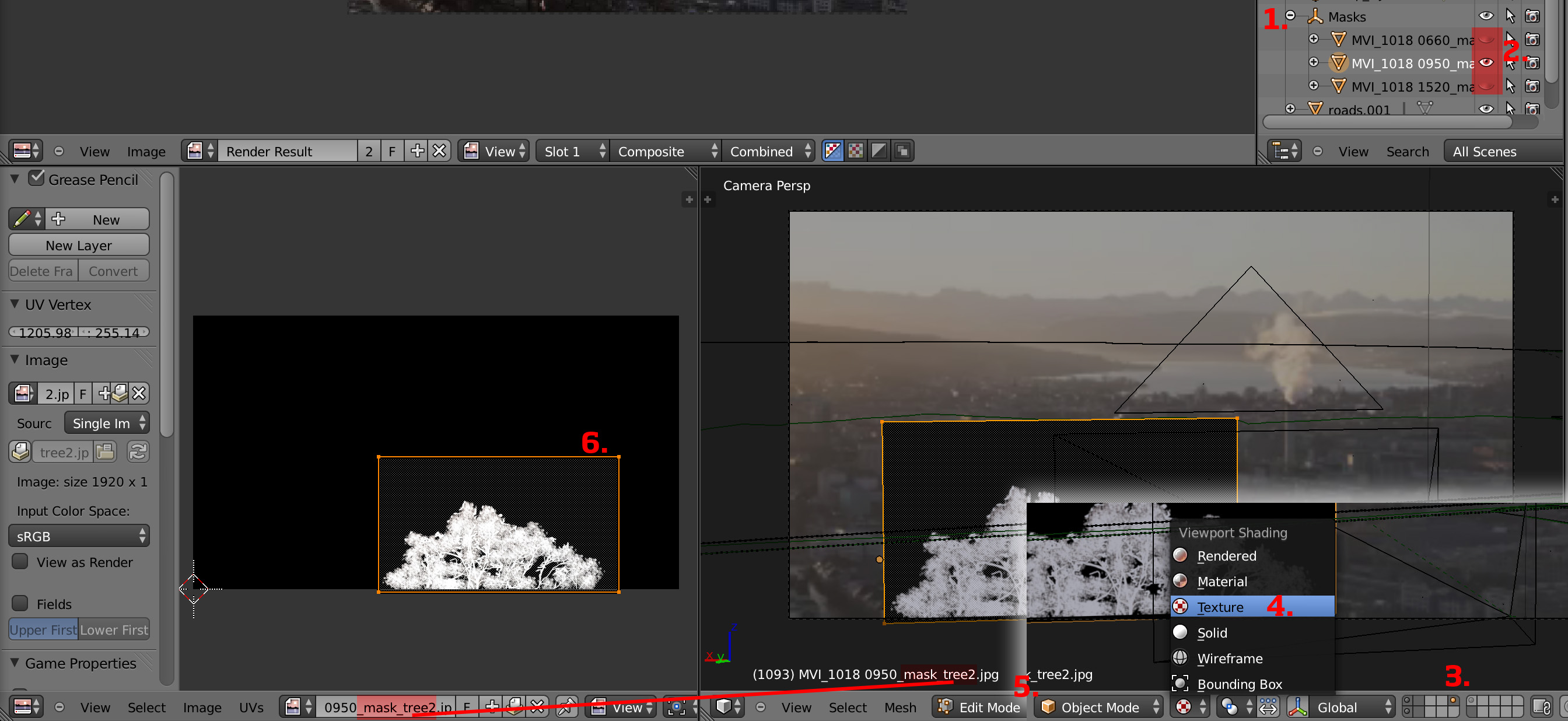
Since it would be a bit tedious to draw the mask for a tree with all its branches it is easier to mask it with a black’n’white image than can be created in Photoshop. In the “Compositing Layout” have a look at the Image window. The tree masks are packed to the .blend file, that’s why you will not find separate image files of the tree masks in the zip file. The symbol showing a white document in a yellow box (2) indicates, that the image files are packed to your .blend file. Click on it, if you want to unpack it. To view all the textures in the file choose another textures from the drop up menu (3).
 These textures are mounted on a vertical panel (a Blender “Plane” Object) in front of the camera. The size of the plane and the size of texture that was put on the plane were adjusted manually. To adjust the mapping of a texture (= how a texture fits on the geometry) UV mapping is being used.
To see how all of this works together, make the mask objects visible (1) and select one of them (2) and turn Layer 5 visible by Shift+Left clicking on the fifth tile below the 3D view port (3). Subsequently, change the render mode of the 3D view port to “Textured” (4) and switch to “Edit Mode” (5). Make sure the image window shows the texture that has been set for the object in the 3D view port. All the selected faces in 3D view’s “Edit mode” now appear in the image window as well (6). By manipulating the geometry in the image window you can scale the texture on the plane.
 In order to include the masks of the trees in the rendering, they need to be rendered out on a different “Render Layer” (1). Having a separate render layer that contains only the masks of the trees allows for adding them to the mask group encountered earlier in the compositing view.
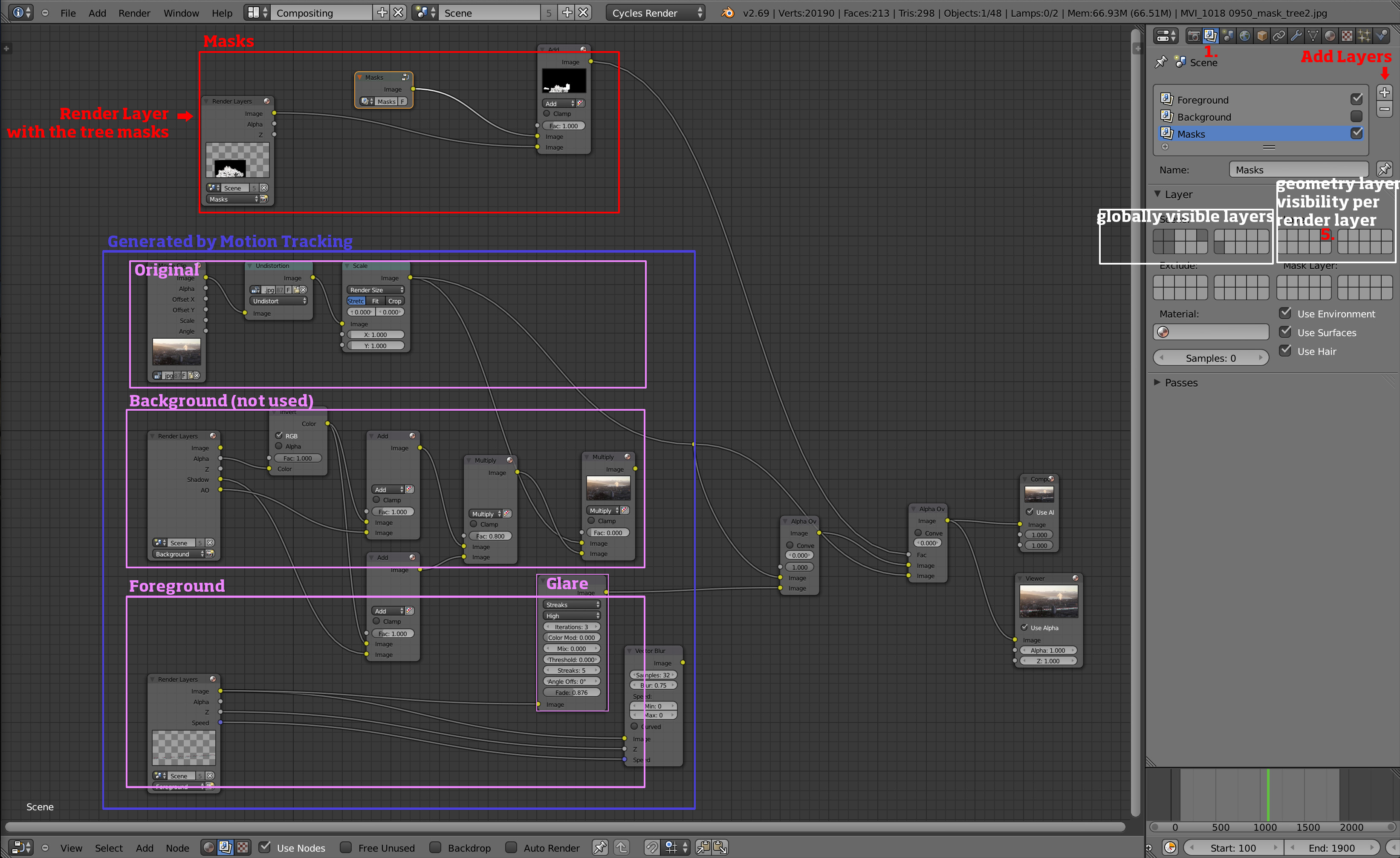 As you can see on the right of the picture above, render layers define which of the globally visible layers should be rendered out to one render layer. In the compositing window the three resulting images “Masks”, “Original”, “Foreground” are composited into one image. This is done for every frame. Think of it as “Photoshopping every frame automatically with visual programming”. For those who know Grasshopper for Rhino: this is like Grasshopper for Photoshop, but using Blender instead of Photoshop.
5. Animated Particle Materials in Cycles
As discussed in this post by Andrew Price you can use the “Particle Info” node to visualize certain properties of your particles in your rendering. Similar to the compositing view, materials in cycles can be edited with a visual node setup. To do so choose the “Material View” in the node editor (2) and select an object (1) the material of which you want to edit.
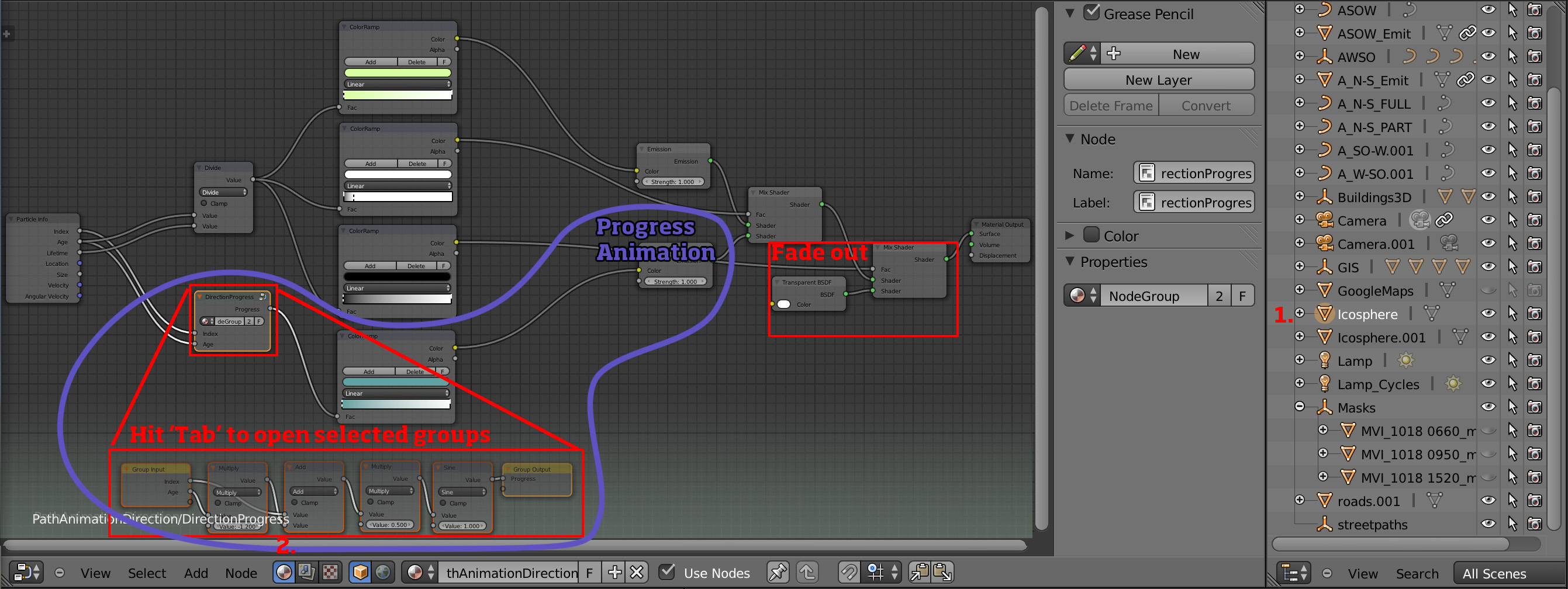 In the path animation material the age and index of a particle get multiplied with a sinus and some other numbers (found by trial n’ error).
6. Putting the streets onto the topography
Included in the .blend file you will find a python script called “vertices2topography.py”. It shows you how to use a ray cast function from python. The function is compiled into Blender, written in C, and much faster therefore much faster, as if it would have been written in python – just for the nerds, but good to know. Ray casting normally is rather computation intense, so knowing you’re not given a bloody toy but a cutting edge tool for the task helps a lot. For copyright reasons the topography and the buildings you see in the image below could not be integrated in the .blend file. Nevertheless there are several ways to get a rough estimation of a topography (through Google Sketch Up for instance) and then use it in combination with that script to put the buildings and the streets onto the topography.
 A model of Zurich viewed from north west looking towards Lake Zurich and Üetliberg.